Basic Instruction Scheduling
(and Software Pipelining)
RISC: Relegate the Important Stuff to Compilers.
Modern RISC processors change the fundamental relationship between hardware and compilers. Prior to RISC, there was a relatively simple division of responsibilities – the hardware was responsible for low-level performance details, while the compiler was responsible for language translation and high-level "machine-independent" optimizations, such as elimination of common subexpressions. Some compilers put substantial effort into good instruction selection algorithms, but this rarely paid off with genuine performance improvements. In fact, many cases existed where the more complex instructions were slower to execute than a group of simpler ones.
With RISC processors the situation is different. The compiler now has primary responsibility for exploiting the performance features of the hardware, and the hardware relies on smart compilers to generate highly optimized code. Without good quality compilers, RISC architectures don't make sense – this is a hardware/software pact.
At its heart, the RISC "philosophy" is about moving the architecture/implementation boundary down closer to the hardware, exposing key performance features to the compiler so that it can (hopefully) take advantage of them. This philosophy dates back to well before the 1980s – the computers developed at Control Data Corporation in the 1960s, including the CDC-6600 which is often considered to be the first RISC, did not distinguish between architecture and implementation at all, and thus exposed virtually all of their hardware features to compilers.
Chief among these performance features, especially on modern processors, is the organization of the processor's pipelines (see Modern Microprocessors – A 90-Minute Guide!). For high performance to be achieved, the compiler must reorder the instructions in the program to make effective use of the instruction-level parallelism offered by the processor, an optimization called instruction scheduling. A specialized form of this optimization, called software pipelining, is specifically designed to handle simple inner loops.
Exploiting the instruction-level parallelism made available by aggressive superscalar and VLIW processors is one of the hottest topics in the compiler community today. Due to the limited size of basic blocks, aggressive schedulers must invariably schedule instructions across branches. A large amount of research has been undertaken in this area over the past decade, but we are still far from the point where global instruction scheduling can be considered a solved problem. This introductory paper will therefore only cover the basics of instruction scheduling for straight-line code sequences such as basic blocks.
The Instruction Scheduling Problem
The problem facing an instruction scheduler is to reorder machine-code instructions to minimize the total number of cycles required to execute a particular instruction sequence. Unfortunately, sequential code executing on a pipelined processor inherently contains dependencies between some instructions. Any transformations performed during instruction scheduling must preserve these dependencies in order to maintain the logic of the code being scheduled.
In addition, instruction schedulers often have a secondary goal of minimizing register lifetimes, or at least not extending them unnecessarily. This is usually a conflicting objective in practice, because limiting the number of live registers introduces false dependencies (more on this later).
Prior to RISC, this problem did exist – instruction scheduling is essentially the same problem as microcode compaction, with some slight differences (microcode compaction and instruction scheduling for a VLIW machine are exactly the same problem). Microcode compaction was used to take a correct vertical sequence of micro-operations and combine these into wider and more parallel horizontal micro-instructions where possible. Two operations could be combined if there were no data dependencies between them and the micro-instruction encoding (format) supported such a combination. In contrast, instruction scheduling only alters the vertical code sequence, and does not explicitly combine operations into groups (except on a VLIW architecture).
Because of the overlap of the execution of instructions in a pipeline structure, the results of an instruction issued in cycle i will not be available until cycle i+n, where n is the length of the appropriate pipeline constraint (ie: the latency of the instruction). If an instruction issued between cycles i and i+n attempts to reference the result of the instruction issued at cycle i, a data dependency has been broken. An interlocked pipeline will detect this situation and stall the execution of the offending instruction until cycle i+n, wasting valuable processor cycles. Even worse, on a pipeline without interlocks the code will produce incorrect results, since the value being referenced will be the result of some other operation!
Automatically finding an optimal schedule for a code sequence can be shown to be NP-complete in its most general form (with arbitrary pipeline constraints), since all legal schedules must be examined to determine the optimal one. Even in a restricted form, with fixed-length latencies of two cycles, the scheduling problem seems to remain intractable [PalemSimons1990] (a weaker NP-completeness proof was presented in [HennessyGross1983], but this proof now appears to be flawed). It is only in the case of single cycle pipeline delays that the problem is optimally solvable in less than exponential time, and in this case linear-time solutions are possible [BernsteinGertner1989], [ProebstingFischer1991].
Although this simple, linear-time case is sufficient for the integer units of the original RISC processors (with their delayed loads and branches), it is inadequate for even the most basic floating-point units, and certainly not suitable for superscalar or VLIW processors (in the early days of the RISC era, most assemblers automatically performed simple linear-time instruction scheduling within basic blocks, until it became obvious that more aggressive scheduling was needed). In many situations, an exhaustive search strategy is actually a viable approach for small code sequences, and is often used by production compilers under restricted conditions (or more precisely, a branch-and-bound search is used, which is effectively a smarter exhaustive search). For larger code blocks, exhaustive search quickly becomes impractical, but heuristically-guided scheduling algorithms can achieve very good results, often within 10% of optimality, in almost linear time.
Types of Dependencies
In practice, three types of data dependency need to be considered...
- A true or read-after-write (RAW) dependency occurs when one instruction reads the result written by another. The read instruction must follow the write instruction by a suitable number of cycles for the result to be read without stalling. This is by far the most common type of dependency, and is the natural result of overlapping the execution of dependent instructions.
- An anti or write-after-read (WAR) dependency occurs when one instruction writes over the operand of another. The read instruction must occur before the write instruction by a suitable number of cycles for the value to be safely read without stalling the write instruction. On most pipelines, values are read near the beginning of the pipeline and written near the end, so anti-dependencies normally require the read instruction to simply be issued before the write, or in the same cycle on a superscalar or VLIW processor (a latency of 0). Anti-dependencies between registers are usually only present if scheduling is performed after register allocation, however anti-dependencies for memory accesses are a natural consequence of pipelined execution of sequential code.
- An output or write-after-write (WAW) dependency occurs if two instructions write to the same target, with the result of the logically first instruction never being used (otherwise this would be a true dependency followed by an anti-dependency). Unless the logically first write instruction has side effects, such as writing to a device driver, it is unnecessary and can be removed.
The first two types of dependencies – read-after-write and write-after-read dependencies – are "real" in the sense that they represent the genuine logic of the program. Any write-after-write dependencies are usually artifacts of either the compilation process or structured programming practices, and can often be removed by dataflow optimizations such as dead-code elimination or partial redundancy elimination. The fourth combination – read-after-read – is, of course, not a dependency at all, because two reads can be performed in any order without affecting the result.
In addition to data dependencies, it is important to remember that programs also contain control dependencies which specify the logical structure of the program and the order in which certain operations must be performed. For example, the then part of an if statement should not be executed until the test has been performed, and then only if the test was true. Loops, conditionals, function calls and so on all represent control dependencies. These types of constraints make moving instructions across branches much more complicated than simply reordering instructions within a straight-line code sequence – this is called global instruction scheduling and is not covered in this introductory paper.
Dependency Graphs
Like most scheduling problems, instruction scheduling is usually modeled as a DAG evaluation problem [HennessyGross1983]. Each node in the data dependency graph represents a single machine instruction, and each arc represents a dependency with a weight corresponding to the latency of the relevant instruction...
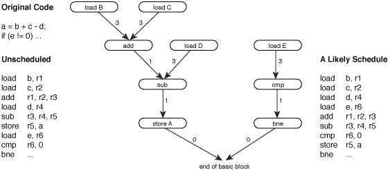
Figure 1 – A data dependency graph.
Resources from which dependencies arise include all forms of storage and any side effects. This includes general, special and status registers, condition codes, and memory locations. Detecting register conflicts is trivial, and condition codes are often handled as if each code were a separate register. Disambiguating memory references, on the other hand, is a very complex issue. Without delving into complex alias analysis, it is clear that certain memory references cannot alias each other – different offsets from the same base register cannot refer to the same location, and memory in the stack cannot overlap with memory in the heap or globals area. Without further alias analysis, conservative assumptions must be made.
Given a dependency graph such as the one shown above, an instruction scheduling algorithm must find an evaluation order for the graph in which all parents are evaluated before their children by at least as many cycles as the weighted links between parent and child. Provided these requirements are met, the semantic properties of the code sequence being scheduled will not change.
If scheduling is performed after or alongside register allocation, there may be two additional conditions – values that were live at the start of the original code sequence remain live at the start of the new code sequence, and values that were live at the end of the original code sequence remain live at the end of the new code sequence. Modern optimizers place instruction scheduling before register allocation, and thus do not have to obey these constraints except during any post- register-allocation reschedule, if necessary.
Labeling memory accesses such as loads with a fixed latency introduces a degree of uncertainty into the dependency graph – the latency of a load instruction is not fixed and will actually vary greatly depending on whether it is a cache hit or not. Many schedulers simply assume a primary data cache hit for every access, basing this assumption on the fact that around 90% of memory accesses are indeed D-cache hits. More sophisticated approaches attempt to allow for the unpredictable nature of memory accesses by distributing the memory operations as evenly as possible [KernsEggers1993], [LoEggers1995].
Control dependencies can be directly represented on a data dependency graph, by conversion to data dependencies, but they are usually handled in an ad-hoc manner by dealing directly with basic block structures and the control flow graph. For now, control flow issues will be ignored (this paper does not cover global instruction scheduling).
Structural hazards, imposed by limitations of the hardware, must also be handled in a special way, since they represent what would be undirected arcs on the graph. For example, two add instructions might use the same hardware, and hence conflict with each other. As a result they cannot proceed simultaneously, but any ordering would avoid this conflict. Such information is usually modeled by timing heuristics or resource reservation tables.
The nodes and edges in a dependency graph are usually annotated with information to help the scheduler decide between ready instructions. Although much of this information can be obtained during graph construction, it is sometimes necessary to perform a separate traversal to obtain information only available when the graph is traversed in the direction opposite to that of creation. For example, if the graph is created in a forward pass then information such as distance-to-end must be obtained by a separate backward traversal. In addition, some information is dynamic in nature and cannot be collected until the actual scheduling pass.
Regardless of the direction of construction, determining which nodes a new node should be connected to can be done in two distinct ways. The easiest method is a compare-against-all approach where every node is checked for dependencies with every other node. Since every node must be compared with every other node except itself, (n2-n)/2 comparisons must be made during graph construction, giving this type of construction a time order of O(n2). Since a potentially large number of nodes may exist (sometimes hundreds or even thousands for global scheduling) this is an unacceptable approach. Nonetheless, many early schedulers did use the compare-against-all approach. Such schedulers gave themselves away by performing extremely slow compilations of the fpppp SPEC benchmark, which has a basic block of 10000 instructions!
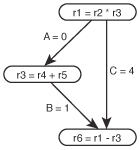
Figure 2 – A necessary
transitive arc.
A more intelligent approach is to track the last instruction to define each machine resource, since only these instructions can conflict with new instructions. These so-called table-building approaches run in time proportional to the number of instructions because the number of machine resources does not vary as instructions are added [SmothermanEtc1991]. They also have other advantages over the compare-against-all approach, the most important being that unnecessary transitive arcs are not created as the graph is constructed.
Some transitive arcs are necessary, however, to maintain the graph's timing constraints. Luckily, the table-building approaches maintain these arcs correctly, because they involve combinations of different types of dependencies. The most common example of a necessary transitive arc is shown on the right – the result of an anti-dependency/true-dependency pair. Even though the order of the instructions would not change if arc C was removed, the apparent path length from the multiply to the subtraction, and hence the apparent latency of the multiply instruction, would appear to be a single cycle. Obviously this is incorrect.
Scheduling Heuristics
There have been many heuristic attacks on the instruction scheduling problem. Most of these have followed the general approach set down by John Hennessy and Thomas Gross in 1983 [HennessyGross1983], which is based on standard list scheduling (another notable approach is the modification of Sethi-Ullman expression evaluation to compensate for some forms of pipeline delays [ProebstingFischer1991], however that approach cannot easily be extended to handle the more complex scheduling problems presented by modern superscalar processors).
List scheduling approaches work by maintaining a ready list which contains all the instructions that can legally be executed at a particular point in time. The scheduler repeatedly chooses an instruction from the ready list, removes it from the list and issues it (inserts it into the final schedule). This in turn makes other instructions ready, and these are added to the list. The key to the whole process is the set of heuristics used to select the best instruction to issue.
In general, scheduling heuristics are used in combinations, called priority functions, to try to select the best instruction to be issued for a particular situation. Although there are literally hundreds of popular heuristics in use today, they can be grouped into a few broad categories [Krishnamurthy1990], [SmothermanEtc1991]...
- Stall Prevention or Instruction Class Heuristics
- Stall prevention heuristics attempt to detect when an instruction will stall if executed at a particular point in time. This typically involves maintaining an earliest execution time for each instruction (or a latest execution time if scheduling is done in a backward direction). Instructions cannot be started before their earliest execution time without stalling. To maintain earliest execution times for each instruction, a current time is maintained by the scheduler and every time an instruction is issued each of its children has its earliest execution time updated to the sum of the current time and the weight of the relevant arc.
- A more flexible approach to detecting stalls is to also compare the instruction class (type) of each ready instruction with that of the last issued instruction (or group of instructions for a superscalar processor). Unfortunately, the use of such a pass adds yet another traversal of instructions to the scheduler, increasing a linear-time algorithm to O(n2). On the other hand, it does provide a degree of flexibility for handling the subtle grouping rules of many superscalar and VLIW processors.
- Hardware resource hazards that relate to the extended (non-pipelined) use of a single resource, such as a floating-point divide unit, can be handled by ad-hoc heuristics or by using explicit resource reservation tables. Some schedulers even consider migrating instructions from one class to another if the desired resources are unavailable but alternate ones can be used. A shift operation, for example, can be converted into a multiply, or the floating-point unit may be used to perform integer operations on values within suitable bounds. The latter approach is better handled by designing the floating-point unit to double as an integer unit [SastryEtc1998].
- Critical Path Heuristics
- As you might expect, critical path heuristics determine which instructions fall on the critical path. Unlike some simpler scheduling problems, instruction scheduling is a resource constrained problem. Thus, an optimal sequence of instructions may be longer than the critical path, and may not issue the instructions on the critical path as early as possible. Since an optimal schedule cannot be shorter than the critical path, these instructions are usually issued relatively early in the schedule simply because they may constrain the total execution time.
- The most useful of the critical path heuristics is length to end – the maximum distance along any path from a particular instruction to the end of the code sequence. A traversal picking the largest length to end at each level of the graph will select the critical path. Since the graph contains no back edges, length to end values for each instruction can be calculated in a trivial backward pass, or during backward graph construction.
- Another method, which requires two passes over the graph, is to calculate both earliest start time and latest start time for each node, then to determine the slack time (latest - earliest) for each instruction. Naturally, instructions with a slack time of zero are on the critical path. Although this is less efficient than calculating the length to end, it does provide "slackness" information which can be used in balancing heuristics. Note that earliest start time is not the same as earliest execution time. Earliest start time is a static measurement of the maximum path length from the leaves, while earliest execution time is a dynamic heuristic maintained by using instruction class information.
- Uncovering or Balancing Heuristics
- Uncovering or balancing heuristics, sometimes called "fairness" heuristics, attempt to balance the progress through the graph by determining how many nodes will be added to the ready list if a particular instruction is issued. Simple approaches include counting the number of children or number of single-parent children of each instruction. More sophisticated methods include calculating total delays to children, number of descendants or total descendant path length. Perhaps the best indicator is the number of uncovered children, a dynamic heuristic which counts the number of children that have only one unissued parent (the node being considered for issuing).
- Register Usage Heuristics
- Register usage heuristics attempt to reduce the live ranges of registers so that later register allocation phases are more successful. A simple example is the calculation of the number of registers born or killed in a particular instruction. A more sophisticated register usage approach is the dynamic promotion of the children of a register-birthing instruction when that instruction is issued. Instead of simply deferring register-birthing instructions until after register-killing ones, this approach attempts to keep the instructions which create, use and destroy a particular register close together. The GNU instruction scheduler uses this heuristic with considerable success.
Software Pipelining
Since a large portion of the execution time of most programs is spent in small inner loops, the schedules chosen for the bodies of these loops are a key factor in the overall performance of many programs. Studies of the structure of inner loops suggest they have a few properties that make them different from other types of code.
Inner loops tend to perform the same kinds of operations on different pieces of data each time around the loop. They normally start by loading some data from memory, then perform a sequence of arithmetic operations on that data, and finally store the results back into memory. Unfortunately, this load-operate-store sequence is not well suited to the relatively long latencies of memory loads found in today's systems. As a result, most loops suffer from a ramp-up effect at the start of each iteration. If long running floating-point operations are being performed, the loop body also tends to suffer from a ramp-down at the end of each iteration.
Such ramp-up/ramp-down behavior significantly reduces the loop's overall throughput, because processor resources are not being fully utilized for the entire duration of the loop...
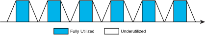
Figure 3 – The ramp-up/ramp-down behavior of many inner loops.
Software pipelining attempts to reduce these ramp-up and ramp-down periods to once before the loop begins and once after it has completed. This is done by rearranging the loop body to overlap instructions from different iterations of the original loop. If parts of k iterations are overlapped, the new loop is executed n-k times, with the loop prolog and epilog making up the remaining k iterations.
Alone, or more often in combination with loop unrolling, this maximizes the amount of useful work done per cycle during the loop...
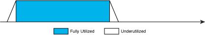
Figure 4 – Reducing the ramp-up/ramp-down effect with software pipelining.
Of course, if the loop iterates less than k times at runtime, then the code must not enter the software-pipelined version. Often, a test must be performed beforehand which jumps to an alternative, non-software-pipelined version of the loop in these cases. It is for this reason that many optimizers only perform software pipelining for loops with constant bounds.
Algorithms to achieve software pipelining generally fall into two basic categories...
- algorithms in which the loop is continuously unrolled and scheduled until a point is reached where the schedule can wrap back on itself [NicolauPotasman1990]
- modulo scheduling algorithms which try different staggerings of iterations in an attempt to find a staggering that yields a perfect schedule [Lam1988]
It is generally believed that the first class of algorithms tend to cause an explosion of both code size and optimization time, because a perfectly wrapping schedule may require hundreds of iterations to be unrolled. As a result, most of the research into software pipelining has concentrated on modulo scheduling techniques.
To ensure a tight, repeatable loop body is reached, modulo scheduling algorithms impose two additional constraints on the software pipelining problem...
- the staggering or initiation interval between all iterations must be the same, and
- the schedule for all the individual iterations must be identical
In the presence of these constraints, the modulo scheduling problem is to schedule the operations within an iteration such that the iterations can be overlapped with the shortest initiation interval. Such a schedule is produced by using a special scheduler which is aware of the initiation interval and the resulting loop-carried constraints between iterations...
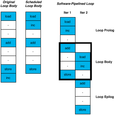
Figure 5 – Software pipelining (modulo scheduling).
The body of the loop is repeatedly scheduled with different initiation intervals until a perfect schedule is reached [Lam1988], [AikenNicolau1988]. Only a relatively small number of intervals need to be considered, since an upper bound on the initiation interval is the length of the unscheduled loop body and a lower bound is the longest loop-carried dependency. In addition, it is often possible to find a perfect schedule at or near the lower bound, making the process faster in practice than it might appear.
Although the above example is for a single issue processor, in practice software pipelining is of most benefit for superscalar and VLIW processors. With luck, several different iterations can be overlapped and a wide set of instructions can execute the entire loop body in a single cycle. Thus, the above loop might be able to be executed at the rate of one cycle per iteration on a 4-issue superscalar processor that supported one integer and one floating-point instruction, plus two memory operations (one load and one store) per cycle. Unfortunately, more detailed examination reveals a flaw – such a schedule would not be possible without introducing some new register-to-register move instructions to "shuffle" the data from one iteration to the next. Thus, an even wider processor would be required, or the optimizer would need to unroll the loop a suitable number of times so that the shuffling was unnecessary (Intel's IA64 architecture provides a novel hardware feature – a rotating register set – to help avoid this problem). In practice, however, it is possible to schedule this loop (with 3x unrolling) so that it executes in 2 cycles per iteration on existing superscalar and VLIW processors supporting a single memory operation per cycle.
In this example we have ignored the final loop branch for simplicity. Under some conditions, the inc instruction could be converted into an operate-test-and-branch instruction, like the PowerPC decrement-and-branch CTR instructions. Such instructions do have genuine benefits for software pipelining situations, sometimes making a 3-issue processor (such as the PowerPC G3/G4) match a 4-issue processor without such an instruction (such as UltraSPARC or Alpha 21164).
As mentioned above, software pipelining is almost always applied in concert with loop unrolling, further increasing the potential for exploiting parallelism. This combination has been shown to be remarkably effective in practice. In one famous "showdown" experiment, the heuristically-guided MIPS software pipeliner was compared to an exhaustive search scheduler which always found the optimal loop schedule. In all of the SPEC92 benchmarks, the optimal scheduler was only able to improve on the MIPS scheduler for a single loop, despite taking 3000 times the amount of optimization time [RuttenbergEtc1996].
Unfortunately, due to its restricted nature, a loop modulo scheduler can only understand very simple loop bodies, which restricts its use to simple inner loops. Any branches, or indeed other complexities such as complex loop termination tests, may prevent modulo scheduling from being applied, forcing the optimizer to fall back to loop unrolling (only). This may still allow the overlap of some of the operations from multiple iterations, but usually it cannot completely avoid the ramp-up/ramp-down problem. The availability of conditional move instructions in the target architecture, with their ability to eliminate conditional branches, can be a critical factor in determining whether software pipelining can be applied to inner loops containing conditional branches (this is one of the main reasons behind IA64's almost fully predicated instruction set).
One approach to solving this problem is hierarchical reduction, where small inner conditionals are grouped into special meta-nodes in the dependency graph which are then treated as if they were a single complicated instruction in an otherwise straight-line code sequence [Lam1988]. Unless both sides of the conditional are of identical length and have the same scheduling characteristics, this necessarily involves a loss of precision – using a conservative approximation of the combined scheduling characteristics of both sides usually leads to "holes" in processor utilization at runtime on one side of the conditional or the other.
Another approach to solving this deficiency, and extending software pipelining's applicability, is circular scheduling [Jain1991]. Instead of considering arbitrary numbers of simple loop bodies all identically scheduled and evenly overlapped, a circular scheduler (sometimes called a window scheduler due to the way they are often implemented) works with a single body like a normal scheduler, but has the power to selectively move instructions from the start of one iteration into the end of the previous iteration – in effect, achieving what a programmer might call ahead-by-one calculation. The new loop body is then rescheduled to see if an improvement has been made. In addition to being relatively simple to implement (for a restricted set of situations), circular scheduling effectively allows the second iteration to be scheduled differently from the first – something modulo scheduling does not permit. This allows the scheduler to be more flexible in the decisions it makes, which may be unimportant for highly parallel code but is of great importance when parallelism is scarce.
Register Allocation – A Phase Ordering Problem
Instruction scheduling is usually performed before register allocation, when the structure of the final code has been determined but specific register usage has yet to be decided. Unfortunately, this ordering of the two optimizations can cause problems, since any spill code which needs to be inserted by the register allocator may not get the full benefit of the instruction scheduler's attention (or even worse, the new code may disrupt the schedule provided by the scheduler).
It is possible to perform instruction scheduling after register allocation, but such approaches place tremendous restrictions on what the scheduler can achieve, because the register allocation process introduces many artificial anti-dependencies between instructions. This is a classic phase ordering problem.
To demonstrate the problem, consider the following code sequence, which is used as a trivial example in the Register Allocation by Graph Coloring introductory paper. On the left, the code sequence is shown before scheduling and register allocation, and with its scheduled equivalent. All four assignments can be done in parallel, as can all four uses. On the right, the same code sequence is shown but register allocation has already been applied. Once aggressive graph coloring register allocation has occurred there is much less parallelism available (only half as much)...
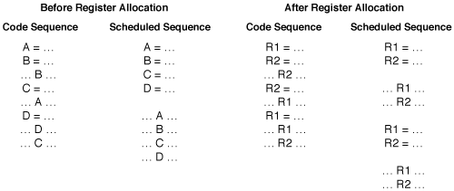
Figure 6 – Register allocation hampers instruction scheduling.
Attempts have been made to integrate register allocation and instruction scheduling into a single optimization [Pinter1993]. Unfortunately, this is difficult to do and the resulting algorithms are often complex and restrictive. In practice, there are many benefits in separating these two optimizations so that the best available algorithms can be used for each problem. Thus, most production compilers use a combination of reinvoking the instruction scheduler a second time after register allocation, and enhancing the scheduler to show a degree of restraint in an attempt to avoid extending register lifetimes unnecessarily. Often, this "restraint" is in the form of either an heuristic (as mentioned above) or an upper limit on the number of live registers allowed for each basic block [GoodmanHsu1988], [BradleeEtc1991]. Another alternative is to perform an additional pass to reduce register pressure after aggressive scheduling [ChenSmith1999].
More Information?
The best way to learn about instruction scheduling is to write a simple instruction scheduler yourself. Simple schedulers are surprisingly easy to write, and the heuristics mentioned above, and in more detail in papers such as [Krishnamurthy1990] and [SmothermanEtc1991], then take on much more relevance.
More aggressive schedulers invariably need to schedule instructions across branches. Many alternative strategies have been proposed to achieve this, ranging from approaches that attempt to preserve the feel of a sequential code sequence from the scheduler's point of view, such as trace scheduling, superblocks and hyperblocks, through to approaches which explicitly attack the global nature of the problem by using control dependence graphs and dominance relationships. In my opinion, the following four documents best introduce this spectrum of approaches: the PhD thesis of John Ellis describes the motivation and techniques of trace scheduling; Scott Mahlke's PhD thesis describes superblocks, hyperblocks and predication; Michael Smith's PhD thesis describes a more global approach; and the SIGPLAN '91 PLDI paper by David Bernstein and Michael Rodeh [BernsteinRodeh1991] describes the fully global approach based on the control dependence graph.
Instruction scheduling and software pipelining are also covered in some detail, although global scheduling techniques are only covered superficially, in the book "Advanced Compiler Design & Implementation" by Steven Muchnick [Muchnick1997].